Examples
This page shows application examples with open sections, sections with branches, closed sections, multi-cells, booms and shear connectors. You can also locate these examples as individual modules in the abdbeam.examples package.
Contents
Kollár/Springer C-Section Example
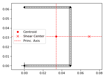
Open sections are the simplest and most common beam type. In this C-Section example from ref. [1], we calculate, print and plot section properties, create a load case with a vertical shear of 100N and plot its Nxy internal loads. Units for this problem are: m, N and Pa:
import abdbeam as ab
sc = ab.Section()
# Create a materials dictionary:
mts = dict()
mts[1] = ab.Laminate()
mts[1].ply_materials[1] = ab.PlyMaterial(0.0001, 148e9, 9.65e9, 4.55e9,
0.3)
mts[1].ply_materials[2] = ab.PlyMaterial(0.0002, 16.39e9, 16.39e9,
38.19e9, 0.801)
mts[1].plies = [[0,2], [0,2], [0,1], [0,1],
[0,1], [0,1], [0,1], [0,1]]
mts[1].symmetry = 'S'
# Create a points dictionary based on Y and Z point coordinates:
pts = dict()
pts[1] = ab.Point(0.0, 0.0)
pts[2] = ab.Point(0.049, 0.0)
pts[3] = ab.Point(0.049, 0.062)
pts[4] = ab.Point(0.0, 0.062)
# Create a segments dictionary referencing point and material ids:
sgs = dict()
sgs[1] = ab.Segment(1,2,1)
sgs[2] = ab.Segment(2,3,1)
sgs[3] = ab.Segment(3,4,1)
# Point the dictionaries to the section
sc.materials = mts
sc.points = pts
sc.segments = sgs
# Calculate and output section properties
sc.calculate_properties()
sc.summary()
ab.plot_section(sc, figsize=(6.4*0.8, 4.8*0.8))
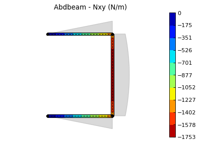
# Create a single load case and calculate its internal loads
sc.loads[1] = ab.Load(Vz_s=-100)
sc.calculate_internal_loads()
# Plot internal loads
ab.plot_section_loads(sc, 1, int_load_list=['Nxy'],
title_list=['Abdbeam - Nxy (N/m)'],
figsize=(6.4*0.8, 4.8*0.8))
Which prints:
Section Summary
===============

Number of points: 4
Number of segments: 3
Number of cells: 0

Centroid
--------
yc     = 3.39937500e-02
zc     = 3.10000000e-02

Shear Center
------------
ys     = 6.92284048e-02
zs     = 3.10000000e-02

Replacement Stiffnesses
-----------------------
EA     = 3.08687460e+07
EIyy   = 2.20044020e+04
EIzz   = 8.18260398e+03
EIyz   = 3.72546093e-12
GJ     = 1.31941376e+01
EImax  = 2.20044020e+04
EImin  = 8.18260398e+03
Angle  = -1.54432286e-14

[P_c] - Beam Stiffness Matrix at the Centroid
---------------------------------------------
[[ 3.08687460e+07  2.87672843e-10 -1.44055909e-10  0.00000000e+00]
 [ 2.87672843e-10  2.20044020e+04  3.72546093e-12  0.00000000e+00]
 [ 1.45837431e-10  5.47177645e-12  8.18260398e+03  0.00000000e+00]
 [ 0.00000000e+00  0.00000000e+00  0.00000000e+00  1.31941376e+01]]

[W_c] - Beam Compliance Matrix at the Centroid
----------------------------------------------
[[ 3.23952259e-08 -4.23516474e-22  5.70322567e-22  0.00000000e+00]
 [-4.23516474e-22  4.54454522e-05 -2.06908775e-20  0.00000000e+00]
 [-5.77375679e-22 -3.03897581e-20  1.22210485e-04  0.00000000e+00]
 [ 0.00000000e+00  0.00000000e+00  0.00000000e+00  7.57912363e-02]]

[P] - Beam Stiffness Matrix at the Origin
-----------------------------------------
[[3.08687460e+07 9.56931125e+05 1.04934443e+06 0.00000000e+00]
 [9.56931125e+05 5.16692669e+04 3.25296774e+04 0.00000000e+00]
 [1.04934443e+06 3.25296774e+04 4.38537563e+04 0.00000000e+00]
 [0.00000000e+00 0.00000000e+00 0.00000000e+00 1.31941376e+01]]

[W] - Beam Compliance Matrix at the Origin
------------------------------------------
[[ 2.17291691e-07 -1.40880902e-06 -4.15439267e-06  0.00000000e+00]
 [-1.40880902e-06  4.54454522e-05 -2.06908775e-20  0.00000000e+00]
 [-4.15439267e-06 -3.03897581e-20  1.22210485e-04  0.00000000e+00]
 [ 0.00000000e+00  0.00000000e+00  0.00000000e+00  7.57912363e-02]]
And plots:
Back to Contents.
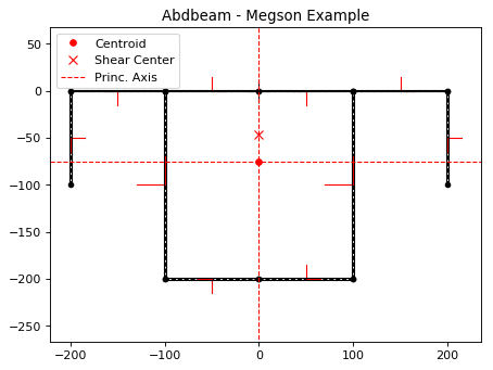
Megson’s Closed Section with Branches Example
Megson’s book (ref [2]) example 19.1 is dedicated to calculating the shear flow distribution for a beam combining open and closed section elements. Units for this problem are: mm, N and MPa.
We start creating the section and calculating its properties:
import abdbeam as ab

sc = ab.Section()
# Create a dictionary for the isotropic material
mts = dict()
mts[1] =  ab.Isotropic(2, 70000, 0.3)
# Create a points dictionary based on Y and Z point coordinates
pts = dict()
pts[1] = ab.Point(0,-200)
pts[2] = ab.Point(-100,-200)
pts[3] = ab.Point(-100,0)
pts[4] = ab.Point(-200,0)
pts[5] = ab.Point(-200,-100)
pts[6] = ab.Point(0,0)
pts[7] = ab.Point(100,-200)
pts[8] = ab.Point(100,0)
pts[9] = ab.Point(200,0)
pts[10] = ab.Point(200,-100)
# Create a segments dictionary referencing point and material ids
sgs = dict()
sgs[1] = ab.Segment(1,2,1)
sgs[2] = ab.Segment(2,3,1)
sgs[3] = ab.Segment(3,4,1)
sgs[4] = ab.Segment(4,5,1)
sgs[5] = ab.Segment(3,6,1)
sgs[6] = ab.Segment(1,7,1)
sgs[7] = ab.Segment(7,8,1)
sgs[8] = ab.Segment(8,9,1)
sgs[9] = ab.Segment(9,10,1)
sgs[10] = ab.Segment(8,6,1)
# Point the dictionaries to the section
sc.materials = mts
sc.points = pts
sc.segments = sgs
# Calculate section properties
sc.calculate_properties()
Next, we are going to plot the section showing its segments’ orientations, as they are essential to understand shear signs:
# Plot the section
ab.plot_section(sc, segment_coord=True, title='Abdbeam - Megson Example')
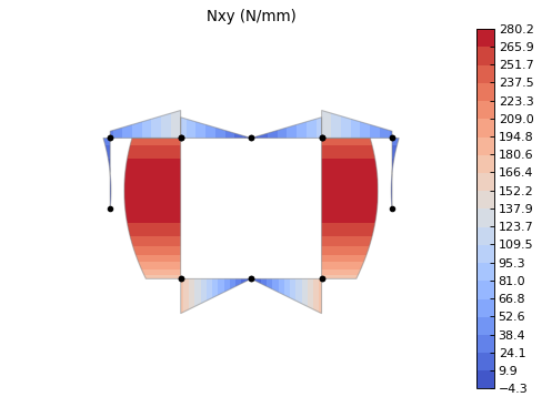
Abdbeam by default plots positive diagrams towards the top side of the laminate and negative diagrams towards the bottom side. To change individual diagram directions, the parameter diagram_factor_list can be used with factors 1.0 or -1.0 as desired. This is also a rather large cross section with thin laminates, so ploting a countour inside the thickness will be hardly visible. To provide a clearer internal load view, we’ll use a contour diagram:
#Create load case and calculate its internal loads:
sc.loads[1] = ab.Load(Vz_s=100000)
sc.calculate_internal_loads()
ab.plot_section_loads(sc, 1, segment_contour=False, diagram=True,
                      diagram_contour=True, diagram_alpha=1.0,
                      contour_levels=20, contour_color='coolwarm',
                      diagram_factor_list=[1,1,-1,-1,1,-1,-1,1,1,-1],
                      thickness=False, int_load_list=['Nxy'],
                      title_list=['Nxy (N/mm)'])
Back to Contents.
Kollár/Springer Single Cell Example
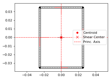
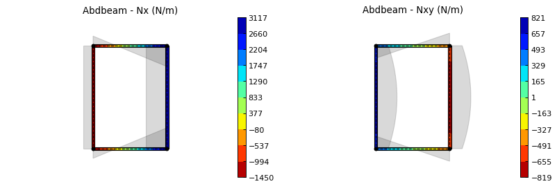
In this single rectangular cell example from ref. [1], the laminate is asymmetric. This requires special attention when defining the point connectivity of each segment, so that the bottom and top plies are at their intended sides. We’ll calculate, print and plot section properties, create a load case with combined external loads and plot its Nx and Nxy internal loads in a single plot. Units for this problem are: m, N and Pa:
import abdbeam as ab

sc = ab.Section()
# Create a materials dictionary:
mts = dict()
mts[1] = ab.Laminate()
mts[1].ply_materials[1] = ab.PlyMaterial(0.0001, 148e9, 9.65e9, 4.55e9,
                                         0.3)
mts[1].ply_materials[2] = ab.PlyMaterial(0.0002, 16.39e9, 16.39e9,
                                         38.19e9, 0.801)
mts[1].plies = [[0,1]]*10 + [[45,1]]*10
mts[1].symmetry = 'T'
# Create a points dictionary based on Y and Z point coordinates:
pts = dict()
pts[1] = ab.Point(-0.025, -0.035)
pts[2] = ab.Point(0.025, -0.035)
pts[3] = ab.Point(0.025, 0.035)
pts[4] = ab.Point(-0.025, 0.035)
# Create a segments dictionary referencing point and material ids:
sgs = dict()
sgs[1] = ab.Segment(1,2,1)
sgs[2] = ab.Segment(2,3,1)
sgs[3] = ab.Segment(3,4,1)
sgs[4] = ab.Segment(4,1,1)
# Point the dictionaries to the section
sc.materials = mts
sc.points = pts
sc.segments = sgs
# Calculate and output section properties
sc.calculate_properties()
sc.summary()
ab.plot_section(sc, segment_coord=True, figsize=(6.4*0.8, 4.8*0.8))
# Create a single load case and calculate its internal loads
sc.loads[1] = ab.Load(Px=200, Mz=10, Vz_s=-100)
sc.calculate_internal_loads()
# Plot internal loads
ab.plot_section_loads(sc, 1, int_load_list=['Nx', 'Nxy'],
                      title_list=['Abdbeam - Nx (N/m)',
                      'Abdbeam - Nxy (N/m)'], figsize=(6.4*0.8, 4.8*0.8))
Which prints:
Section Summary
===============

Number of points: 4
Number of segments: 4
Number of cells: 1

Centroid
--------
yc     = 0.00000000e+00
zc     = 0.00000000e+00

Shear Center
------------
ys     = 0.00000000e+00
zs     = -6.93889390e-19

Replacement Stiffnesses
-----------------------
EA     = 3.99342118e+07
EIyy   = 2.94941190e+04
EIzz   = 1.79757984e+04
EIyz   = 0.00000000e+00
GJ     = 4.10520186e+03
EImax  = 2.94941190e+04
EImin  = 1.79757984e+04
Angle  = -0.00000000e+00

[P_c] - Beam Stiffness Matrix at the Centroid
---------------------------------------------
[[ 3.99342118e+07 -0.00000000e+00 -0.00000000e+00  6.75301020e+04]
 [ 0.00000000e+00  2.94941190e+04  0.00000000e+00  0.00000000e+00]
 [ 0.00000000e+00  0.00000000e+00  1.79757984e+04  0.00000000e+00]
 [ 6.75301020e+04  0.00000000e+00  0.00000000e+00  4.10520186e+03]]

[W_c] - Beam Compliance Matrix at the Centroid
----------------------------------------------
[[ 2.57576953e-08  0.00000000e+00  0.00000000e+00 -4.23711147e-07]
 [ 0.00000000e+00  3.39050642e-05  0.00000000e+00  0.00000000e+00]
 [ 0.00000000e+00  0.00000000e+00  5.56303524e-05  0.00000000e+00]
 [-4.23711147e-07  0.00000000e+00  0.00000000e+00  2.50563381e-04]]

[P] - Beam Stiffness Matrix at the Origin
-----------------------------------------
[[ 3.99342118e+07 -0.00000000e+00 -0.00000000e+00  6.75301020e+04]
 [ 0.00000000e+00  2.94941190e+04  0.00000000e+00  0.00000000e+00]
 [ 0.00000000e+00  0.00000000e+00  1.79757984e+04  0.00000000e+00]
 [ 6.75301020e+04  0.00000000e+00  0.00000000e+00  4.10520186e+03]]

[W] - Beam Compliance Matrix at the Origin
------------------------------------------
[[ 2.57576953e-08  0.00000000e+00  0.00000000e+00 -4.23711147e-07]
 [ 0.00000000e+00  3.39050642e-05  0.00000000e+00  0.00000000e+00]
 [ 0.00000000e+00  0.00000000e+00  5.56303524e-05  0.00000000e+00]
 [-4.23711147e-07  0.00000000e+00  0.00000000e+00  2.50563381e-04]]
And plots:
Back to Contents.
Bruhn’s Multi-celled Example
Most idealized solutions to aerospace beam problems assume that booms are connected to segments that can only resist shear. Shear connectors can be used to achieve this, since they only use as inputs a material shear modulus and its thickness.
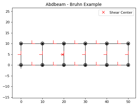
Consider the cross section with 5 cells from Bruhn’s example A15.12 (ref [3]). Two important assumptions are made: the cells segments (beam walls) can only resist shear and the points (beam flanges) develop all the bending resistance. As stated above, in Abdbeam we can enforce these assumptions by modeling the segments with shear connector materials and the section points with EA and/or GJ properties (booms). A Vz load of 1000lbf is applied to the section and only the shear flows (Nxy) at the segments and and shear center are of interest. Units for this problem are: in, lbf and psi.
We’ll start creating the section, calculating its properties and plotting its section. Notice that booms are represented with additional circles around points:
import abdbeam as ab

sc = ab.Section()
# Create a dictionary for the shear connector materials
mts = dict()
mts[1] =  ab.ShearConnector(0.03, 3846154)
mts[2] =  ab.ShearConnector(0.04, 3846154)
mts[3] =  ab.ShearConnector(0.05, 3846154)
mts[4] =  ab.ShearConnector(0.064, 3846154)
# Create a points dictionary based on Y and Z point coordinates
pts = dict()
pts[1] = ab.Point(0,0,2e7,0,'a')
pts[2] = ab.Point(10,0,1e7,0,'b')
pts[3] = ab.Point(20,0,5e6,0,'c')
pts[4] = ab.Point(30,0,5e6,0,'d')
pts[5] = ab.Point(40,0,5e6,0,'e')
pts[6] = ab.Point(50,0,1e7,0,'f')
pts[11] = ab.Point(0,10,2e7,0,'a_')
pts[12] = ab.Point(10,10,1e7,0,'b_')
pts[13] = ab.Point(20,10,5e6,0,'c_')
pts[14] = ab.Point(30,10,5e6,0,'d_')
pts[15] = ab.Point(40,10,5e6,0,'e_')
pts[16] = ab.Point(50,10,1e7,0,'f_')
# Create a segments dictionary referencing point and material ids
sgs = dict()
sgs[1] = ab.Segment(1,2,2,'Bottom 1')
sgs[2] = ab.Segment(2,3,2,'Bottom 2')
sgs[3] = ab.Segment(3,4,2,'Bottom 3')
sgs[4] = ab.Segment(4,5,1,'Bottom 4')
sgs[5] = ab.Segment(5,6,1,'Bottom 5')
sgs[11] = ab.Segment(11,12,2,'Top 1')
sgs[12] = ab.Segment(12,13,2,'Top 2')
sgs[13] = ab.Segment(13,14,2,'Top 3')
sgs[14] = ab.Segment(14,15,1,'Top 4')
sgs[15] = ab.Segment(15,16,1,'Top 5')
sgs[21] = ab.Segment(1,11,4,'Web 1')
sgs[22] = ab.Segment(2,12,3,'Web 2')
sgs[23] = ab.Segment(3,13,2,'Web 3')
sgs[24] = ab.Segment(4,14,2,'Web 4')
sgs[25] = ab.Segment(5,15,1,'Web 5')
sgs[26] = ab.Segment(6,16,1,'Web 6')
# Point the dictionaries to the section
sc.materials = mts
sc.points = pts
sc.segments = sgs
# Calculate section properties
sc.calculate_properties()
# Plot the section
ab.plot_section(sc, centroid =False, princ_dir=False, thickness=False,
                segment_coord=True, title='Abdbeam - Bruhn Example')
Next we’ll create the load case, calculate its internal loads and obtain the shear flows accessing the internal loads Pandas dataframe sc.sgs_int_lds_df directly. Since the segments develop no bending resistance, the shear flow between adjacent points will be constant, and the average Nxy per segment is appropriate:
#Create load case and calculate its internal loads:
sc.loads[1] = ab.Load(Vz_s=1000)
sc.calculate_internal_loads()
# Print the shear flows Nxy for all segments
df = sc.sgs_int_lds_df
print(df[[('Segment_Id', ''),('Nxy','Avg')]])
# Print the shear center location
print('')
print('Shear center is at y = {:.8e}'.format(sc.ys))
Which prints:
   Segment_Id        Nxy
                     Avg
0           1   2.878645
1           2   2.096924
2           3   0.210851
3           4  -1.253519
4           5  -2.586107
5          11  -2.878645
6          12  -2.096924
7          13  -0.210851
8          14   1.253519
9          15   2.586107
10         21  33.484992
11         22  18.963538
12         23  10.976982
13         24  10.555279
14         25  10.423497
15         26  15.595711

Shear center is at y = 1.93602680e+01
Back to Contents.
Torque-box Example
Shear connectors can also be used to model mechanical or bonded joints. This allows the representation of multiple elements of a cross section by their mid-surfaces, usually at the price of creating additional small enclosed areas (cells) between pairs of adjacent shear connector segments.
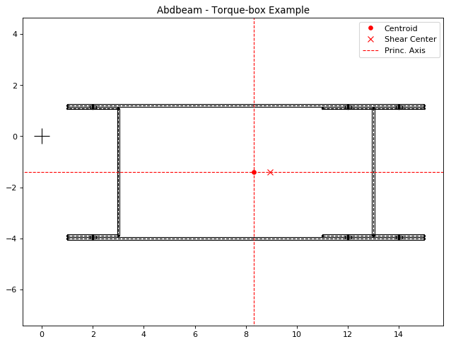
In this example, we create a torque-box using this modeling approach, which could be extended to complex cross sections such as those found in wings, vertical stabilizers, horizontal stabilizers and others (to use aerospace examples). Here we have a C-Section forward spar and a I-Section rear spar with rows of fasteners (shear connectors) connecting them to top and bottom skins. Notice that this modeling approach added two additional closed cells near the rear spar (see the Hat Stiffener Example for a more detailed discussion on the effects of such small closed cells in the section torsional stiffness). Units for this problem are: in, lbf and psi.
First we create the cross section, calculate is properties and plot it:
import abdbeam as ab

sc = ab.Section()
# Create a dictionary to store ply materials shared by laminates
ply_mts = dict()
ply_mts[1] = ab.PlyMaterial(0.0075, 1.149e7, 1.149e7, 6.6e5, 0.04)
# Create the materials dictionary for the laminates and shear connector:
mts = dict()
mts[1] = ab.Laminate()
mts[1].ply_materials[1] = ply_mts[1]
mts[1].plies = [[45,1], [-45,1]]*2 + [[0,1]]*3
mts[1].symmetry = 'S'
mts[2] = ab.ShearConnector(0.25, 6381760)
# Create a points dictionary based on Y and Z point coordinates:
pts = dict()
pts[1] = ab.Point(1,-4)
pts[2] = ab.Point(2,-4)
pts[3] = ab.Point(12,-4)
pts[4] = ab.Point(14,-4)
pts[5] = ab.Point(15,-4)
pts[11] = ab.Point(1,1.21)
pts[12] = ab.Point(2,1.21)
pts[13] = ab.Point(12,1.21)
pts[14] = ab.Point(14,1.21)
pts[15] = ab.Point(15,1.21)
pts[21] = ab.Point(1,-3.895)
pts[22] = ab.Point(2,-3.895)
pts[23] = ab.Point(3,-3.895)
pts[24] = ab.Point(3,1.105)
pts[25] = ab.Point(2,1.105)
pts[26] = ab.Point(1,1.105)
pts[31] = ab.Point(11,-3.895)
pts[32] = ab.Point(12,-3.895)
pts[33] = ab.Point(13,-3.895)
pts[34] = ab.Point(14,-3.895)
pts[35] = ab.Point(15,-3.895)
pts[36] = ab.Point(11,1.105)
pts[37] = ab.Point(12,1.105)
pts[38] = ab.Point(13,1.105)
pts[39] = ab.Point(14,1.105)
pts[40] = ab.Point(15,1.105)
# Create a segments dictionary referencing point and material ids:
sgs = dict()
sgs[1] = ab.Segment(1,2,1,'Bottom Skin')
sgs[2] = ab.Segment(2,3,1,'Bottom Skin')
sgs[3] = ab.Segment(3,4,1,'Bottom Skin')
sgs[4] = ab.Segment(4,5,1,'Bottom Skin')
sgs[11] = ab.Segment(11,12,1,'Top Skin')
sgs[12] = ab.Segment(12,13,1,'Top Skin')
sgs[13] = ab.Segment(13,14,1,'Top Skin')
sgs[14] = ab.Segment(14,15,1,'Top Skin')
sgs[21] = ab.Segment(21,22,1,'Fwd Spar')
sgs[22] = ab.Segment(22,23,1,'Fwd Spar')
sgs[23] = ab.Segment(23,24,1,'Fwd Spar')
sgs[24] = ab.Segment(24,25,1,'Fwd Spar')
sgs[25] = ab.Segment(25,26,1,'Fwd Spar')
sgs[31] = ab.Segment(31,32,1,'Rear Spar')
sgs[32] = ab.Segment(32,33,1,'Rear Spar')
sgs[33] = ab.Segment(33,34,1,'Rear Spar')
sgs[34] = ab.Segment(34,35,1,'Rear Spar')
sgs[35] = ab.Segment(33,38,1,'Rear Spar')
sgs[36] = ab.Segment(36,37,1,'Rear Spar')
sgs[37] = ab.Segment(37,38,1,'Rear Spar')
sgs[38] = ab.Segment(38,39,1,'Rear Spar')
sgs[39] = ab.Segment(39,40,1,'Rear Spar')
sgs[91] = ab.Segment(2,22,2,'Connector')
sgs[92] = ab.Segment(3,32,2,'Connector')
sgs[93] = ab.Segment(4,34,2,'Connector')
sgs[94] = ab.Segment(25,12,2,'Connector')
sgs[95] = ab.Segment(37,13,2,'Connector')
sgs[96] = ab.Segment(39,14,2,'Connector')
# Point the dictionaries to the section
sc.materials = mts
sc.points = pts
sc.segments = sgs
# Calculate section properties
sc.calculate_properties()
# Plot the section
ab.plot_section(sc, pt_size=2, title='Abdbeam - Torque-box Example',
                figsize=(6.4*1.5, 4.8*1.5))
Next we’re going to create 7 load cases with axial, bending, torque and shear loads integrated at the section origin. Yp, zp, ys and zs are then all equal to the default zero and for this reason don’t need to be explicitly entered. Notice that if Px_c were used instead of Px, the axial load would always be assumed to act on the centroid. By using a Px though, a moment arm results from the load application point distance to the calculated centroid. Similarly, if Vy_s and Vz_s were used instead of Vy and Vz, the shear loads would be assumed to always act at the shear center, creating no additional torque in the section. The approach chosen for this example is the typical case for a torque box: loads are integrated at a defined point in space and sizing proceeds changing centroid and shear center locations.
Create the load cases and calculate their internal loads:
# Create load cases and calculate their internal loads
sc.loads[8] = ab.Load(Px=17085,My=-140914,Mz=-7208,Tx=1595,Vy=4727,Vz=-1661)
sc.loads[4] = ab.Load(Px=11854,My=-89211,Mz=-33716,Tx=-57488,Vy=5684,Vz=394)
sc.loads[1] = ab.Load(Px=2395,My=-83206,Mz=210099,Tx=-43162,Vy=1316,Vz=407)
sc.loads[10] = ab.Load(Px=-7458,My=-15571,Mz=-96370,Tx=-3615,Vy=564,Vz=-369)
sc.loads[2] = ab.Load(Px=1000,My=-30865,Mz=180498,Tx=11653,Vy=-7001,Vz=-189)
sc.loads[3] = ab.Load(Px=-281,My=133314,Mz=-123966,Tx=324,Vy=9389,Vz=-1514)
sc.loads[6] = ab.Load(Px=299,My=40658,Mz=101677,Tx=7102,Vy=9214,Vz=-3545)
sc.calculate_internal_loads()
Now let’s say we are analyzing the rear spar and would like to find the critical compressive Nx load among all cases, identify its load case id and segment. Since the calculated internal loads are stored in the Pandas dataframe sc.sgs_int_lds_df, we can use Pandas methods to achieve this:
# Use Pandas methods to get info on the critical spar compressive Nx
df = sc.sgs_int_lds_df
spar_sgs = range(31,40)
df = df[df['Segment_Id'].isin(spar_sgs)]
idx = df[('Nx', 'Min')].idxmin()
min_Nx = round(df.loc[idx, ('Nx', 'Min')],1)
min_sg = int(df.loc[idx, 'Segment_Id'])
min_lc = int(df.loc[idx, 'Load_Id'])
print(('Minimum rear spar Nx is {}, from segment {}, load case {}'
       ).format(min_Nx, min_sg, min_lc))
Which prints:
Minimum rear spar Nx is -1935.9, from segment 34, load case 3
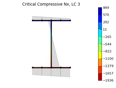
We can finish the example plotting the Nx from this critical load case. To do this, we’re going to filter the rear spar from the rest of the cross section using the parameter plot_sgs and get the load case id from the variable min_lc defined on the previous code block:
# Plot the critical compressive case Nx internal loads
ab.plot_section_loads(sc, min_lc, int_load_list=['Nx'],
                      title_list=['Critical Compressive Nx, LC '+
                      str(min_lc)], plot_sgs=range(31,40),
                      figsize=(6.4*0.8, 4.8*0.8))
Back to Contents.
Hat Stiffener Example
In this example we create a hat stiffner and a skin, both represented at their laminates’ mid-planes. Abdbeam sections cannot have floating segments and we want to capture the hat’s closed cell contribution to the section’s GJ, so we chose here to connect the hat plies to the bottom skin using ShearConnector materials. For these connector’s properties, we entered a t and G that matches compliance term alpha66 (=1/(G*t)) of the skin laminate material.
Notice that, by also connecting the left and right outermost cap points, we added two other cells to the analysis. The areas of these two cells are small and they only increase the total section GJ by 3% (compared to a section removing connectors 91 and 94). Connecting segments that are co-cured or bonded, on the other hand, tend to better represent the Nxy shear distribution in complex sections. This example also shows multiple ways to define a stacking sequence using python lists capabilities. Units for this problem are: in, lbf and psi.
We’ll start creating the section, calculating its properties and showing a summary of these properties:
import abdbeam as ab

sc = ab.Section()
# Create a dictionary to store ply materials shared by laminates
ply_mts = dict()
ply_mts[1] = ab.PlyMaterial(0.0075, 2.147e7, 1.4e6, 6.6e5, 0.3)
ply_mts[2] = ab.PlyMaterial(0.0075, 1.149e7, 1.149e7, 6.6e5, 0.04)
# Create the materials dictionary for the laminates and shear connector:
mts = dict()
mts[1] = ab.Laminate()
mts[1].ply_materials[2] = ply_mts[2]
mts[1].plies = [[45,2], [-45,2]] + [[0,2]]*3
mts[1].symmetry = 'S'
mts[2] = ab.Laminate()
mts[2].ply_materials[2] = ply_mts[2]
mts[2].plies = [[45,2], [-45,2]]*2 + [[0,2]]
mts[2].symmetry = 'S'
mts[3] = ab.Laminate()
mts[3].ply_materials[1] = ply_mts[1]
mts[3].ply_materials[2] = ply_mts[2]
mts[3].plies = [[45,2], [-45,2]] + [[0,1]]*3 + [[0,2]] + [[0,1]]*2
mts[3].symmetry = 'SM'
mts[4] = ab.ShearConnector(0.075, 2605615)
# Create a points dictionary based on Y and Z point coordinates:
pts = dict()
pts[1] = ab.Point(-2, 0)
pts[2] = ab.Point(-1, 0)
pts[3] = ab.Point(1, 0)
pts[4] = ab.Point(2, 0)
pts[5] = ab.Point(-2, 0.075)
pts[6] = ab.Point(-1, 0.075)
pts[7] = ab.Point(-0.35, 0.8)
pts[8] = ab.Point(0.35, 0.8)
pts[9] = ab.Point(1, 0.075)
pts[10] = ab.Point(2, 0.075)
# Create a segments dictionary referencing point and material ids:
sgs = dict()
sgs[1] = ab.Segment(1,2,1,'Skin_Left')
sgs[2] = ab.Segment(2,3,1,'Skin_Center')
sgs[3] = ab.Segment(3,4,1,'Skin_Right')
sgs[10] = ab.Segment(5,6,2,'Hat_Left_Foot')
sgs[11] = ab.Segment(6,7,2,'Hat_Left_Web')
sgs[12] = ab.Segment(7,8,3,'Hat_Top')
sgs[13] = ab.Segment(8,9,2,'Hat_Right_Web')
sgs[14] = ab.Segment(9,10,2,'Hat_Right_Foot')
sgs[91] = ab.Segment(1,5,4,'Connector_1')
sgs[92] = ab.Segment(2,6,4,'Connector_1')
sgs[93] = ab.Segment(3,9,4,'Connector_1')
sgs[94] = ab.Segment(4,10,4,'Connector_1')
# Point the dictionaries to the section
sc.materials = mts
sc.points = pts
sc.segments = sgs
# Calculate section properties
sc.calculate_properties()
sc.summary()
Which prints:
Section Summary
===============

Number of points: 10
Number of segments: 12
Number of cells: 3

Centroid
--------
yc     = 0.00000000e+00
zc     = 2.51301984e-01

Shear Center
------------
ys     = 1.83880688e-16
zs     = 4.13936823e-01

Replacement Stiffnesses
-----------------------
EA     = 5.43010577e+06
EIyy   = 6.22690978e+05
EIzz   = 5.79683101e+06
EIyz   = 7.27595761e-12
GJ     = 2.71545365e+05
EImax  = 5.79683101e+06
EImin  = 6.22690978e+05
Angle  = 8.05702321e-17

[P_c] - Beam Stiffness Matrix at the Centroid
---------------------------------------------
[[ 5.43010577e+06 -1.79003360e-10 -2.09160066e-27  0.00000000e+00]
 [ 0.00000000e+00  6.22690978e+05  7.27595761e-12  0.00000000e+00]
 [ 0.00000000e+00 -1.45519152e-11  5.79683101e+06  0.00000000e+00]
 [ 0.00000000e+00  0.00000000e+00  0.00000000e+00  2.71545365e+05]]

[W_c] - Beam Compliance Matrix at the Centroid
----------------------------------------------
[[ 1.84158476e-07  5.29395592e-23  0.00000000e+00  0.00000000e+00]
 [ 0.00000000e+00  1.60593302e-06 -2.01570488e-24  0.00000000e+00]
 [ 0.00000000e+00  4.03140976e-24  1.72508048e-07  0.00000000e+00]
 [ 0.00000000e+00  0.00000000e+00  0.00000000e+00  3.68262592e-06]]

[P] - Beam Stiffness Matrix at the Origin
-----------------------------------------
[[ 5.43010577e+06  1.36459635e+06 -3.21443370e-27 -0.00000000e+00]
 [ 1.36459635e+06  9.65616750e+05  7.27595761e-12  0.00000000e+00]
 [ 1.36115257e-27 -1.45519152e-11  5.79683101e+06  0.00000000e+00]
 [ 0.00000000e+00  0.00000000e+00  0.00000000e+00  2.71545365e+05]]

[W] - Beam Compliance Matrix at the Origin
------------------------------------------
[[ 2.85577461e-07 -4.03574153e-07  5.06550636e-25  0.00000000e+00]
 [-4.03574153e-07  1.60593302e-06 -2.01570488e-24  0.00000000e+00]
 [-1.01310127e-24  4.03140976e-24  1.72508048e-07  0.00000000e+00]
 [ 0.00000000e+00  0.00000000e+00  0.00000000e+00  3.68262592e-06]]
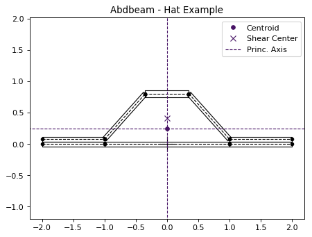
Next, we’ll plot the section hiding segments 91 to 94 (the connectors), since we don’t care about their visual representation:
# Plot the section
ab.plot_section(sc, filter_sgs=[91,92,93,94],
                title='Abdbeam - Hat Example',
                prop_color='#471365')
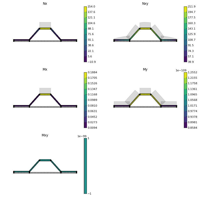
Next, we’ll create two load cases and plot the first case (a rather unusual load case for a stiffener, for ilustration purposes only). Notice that in this plot we listed only the cap segments to show results and continued to filter the connectors:
# Create load cases and calculate their internal loads
sc.loads[1] = ab.Load(My=100, Vy_s=1000)
sc.loads[2] = ab.Load(Tx=100)
sc.calculate_internal_loads()
# Plot internal loads
ab.plot_section_loads(sc, 1, contour_color = 'viridis',
                      result_sgs=[10,11,12,13,14],
                      figsize=(6.4*0.8, 4.8*0.8),
                      diagram_scale=0.5, filter_sgs=[91,92,93,94])
Back to Contents.
References
| [1] | (1, 2) Kollár LP, Springer GS. Mechanics of composite structures. Cambridge university press; 2003 Feb 17. |
| [2] | Megson TH. Aircraft structures for engineering students. Butterworth-Heinemann; 2016 Oct 17. |
| [3] | Bruhn EF, Bollard RJ. Analysis and design of flight vehicle structures. Indianapolis: Jacobs Publishing; 1973 Jun. |