Abdbeam: Composites Cross Section Analysis - Documentation
Abdbeam is a python package for the cross section analysis of thin-walled composite material beams of any shape.
These are a few things you can do with Abdbeam:
- Use a fast thin-walled anisotropic composite beam theory including closed cells, open branches, shear connectors and booms [1];
- Recover replacement stiffnesses (EA, EIyy, EIzz, EIyz, GJ) and/or a full 4 x 4 stiffness matrix for beams with arbitrary layups and shapes;
- Recover centroid and shear center locations;
- Obtain internal load distributions (Nx, Nxy, Mx, My, Mxy for segments; Px and Tx for booms) for a large number of cross section load cases (defined by Px, My, Mz, Tz, Vy and Vz section loads);
- Plot cross sections, their properties and internal loads.
Source Code
The source code is hosted on GitHub at https://github.com/victorazzo/abdbeam.
Quick Example
Let’s use Abdbeam to analyze the cross section with two closed cells below (from [2]):
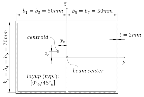
Start creating the section materials, its points and segments (we’ll also calculate the section properties and request a summary at the end):
import abdbeam as ab
sc = ab.Section()
# Create a materials dictionary:
mts = dict()
mts[1] = ab.Laminate()
ply_mat = ab.PlyMaterial(0.166666, 148000, 9650, 4550, 0.3)
mts[1].ply_materials[1] = ply_mat
mts[1].plies = [[0,1]]*6 + [[45,1]]*6
# Create a points dictionary based on Y and Z point coordinates:
pts = dict()
pts[1] = ab.Point(0, -35)
pts[2] = ab.Point(-50, -35)
pts[3] = ab.Point(-50, 35)
pts[4] = ab.Point(0, 35)
pts[5] = ab.Point(50, 35)
pts[6] = ab.Point(50, -35)
# Create a segments dictionary referencing point and material ids:
sgs = dict()
sgs[1] = ab.Segment(1,2,1)
sgs[2] = ab.Segment(2,3,1)
sgs[3] = ab.Segment(3,4,1)
sgs[4] = ab.Segment(4,1,1)
sgs[5] = ab.Segment(4,5,1)
sgs[6] = ab.Segment(5,6,1)
sgs[7] = ab.Segment(6,1,1)
# Point the dictionaries to the section
sc.materials = mts
sc.points = pts
sc.segments = sgs
# Calculate and output section properties
sc.calculate_properties()
sc.summary()
Which prints:
Section Summary
===============

Number of points: 6
Number of segments: 7
Number of cells: 2

Centroid
--------
yc     = -2.67780636e-01
zc     = 0.00000000e+00

Shear Center
------------
ys     = 2.35301214e-03
zs     = -1.45758049e-03

Replacement Stiffnesses
-----------------------
EA     = 6.80329523e+07
EIyy   = 5.24834340e+10
EIzz   = 8.36408748e+10
EIyz   = 0.00000000e+00
GJ     = 1.23762317e+10
EImax  = 8.36408748e+10
EImin  = 5.24834340e+10
Angle  = 0.00000000e+00

[P_c] - Beam Stiffness Matrix at the Centroid
---------------------------------------------
[[ 6.80329523e+07  0.00000000e+00  2.46320132e+05 -1.43701515e+08]
 [ 0.00000000e+00  5.24834340e+10  0.00000000e+00  0.00000000e+00]
 [ 2.46320132e+05  0.00000000e+00  8.36408748e+10 -2.12142163e+07]
 [-1.43701515e+08  0.00000000e+00 -2.12142163e+07  1.23762317e+10]]

[W_c] - Beam Compliance Matrix at the Centroid
----------------------------------------------
[[1.50683149e-08 0.00000000e+00 1.66286490e-28 1.74959530e-10]
 [0.00000000e+00 1.90536313e-11 0.00000000e+00 0.00000000e+00]
 [1.57282135e-25 0.00000000e+00 1.19558821e-11 2.04936911e-14]
 [1.74959530e-10 0.00000000e+00 2.04936911e-14 8.28315446e-11]]

[P] - Beam Stiffness Matrix at the Origin
-----------------------------------------
[[ 6.80329523e+07  0.00000000e+00 -1.79715871e+07 -1.43701515e+08]
 [ 0.00000000e+00  5.24834340e+10  0.00000000e+00  0.00000000e+00]
 [-1.79715871e+07  0.00000000e+00  8.36456213e+10  1.72662667e+07]
 [-1.43701515e+08  0.00000000e+00  1.72662667e+07  1.23762317e+10]]

[W] - Beam Compliance Matrix at the Origin
------------------------------------------
[[1.50691722e-08 0.00000000e+00 3.20155371e-12 1.74965018e-10]
 [0.00000000e+00 1.90536313e-11 0.00000000e+00 0.00000000e+00]
 [3.20155371e-12 0.00000000e+00 1.19558821e-11 2.04936911e-14]
 [1.74965018e-10 0.00000000e+00 2.04936911e-14 8.28315446e-11]]
Now let’s create two load cases (101 and 102) and calculate their internal loads:
sc.loads = dict()
sc.loads[101] = ab.Load(My=5e6)
sc.loads[102] = ab.Load(Tx=250000, Vz=5000.0)
sc.calculate_internal_loads()
Next print all internal loads (which outputs a lot of data we’ll not show here):
sc.print_internal_loads()
Or access the Pandas dataframe containing these internal loads directly:
df = sc.sgs_int_lds_df
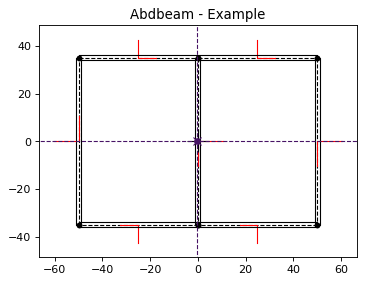
Next plot the cross section and its properties (we’ll show the segment orientations, hide legends, change the centroid, shear center and principal axis colors and use a custom figure size):
ab.plot_section(sc, segment_coord=True, title='Abdbeam - Example',
                legend=False, prop_color='#471365', figsize=(5.12, 3.84))
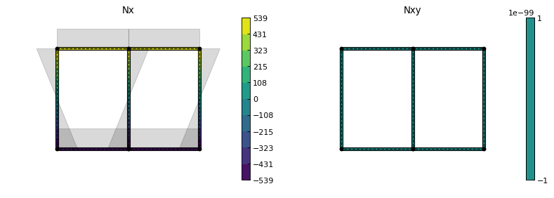
Finally, plot Nx and Nxy for load case 101 (we’ll change the matplotlib contour palette, reduce the internal load diagram scale, and use a custom figure size):
ab.plot_section_loads(sc, 101, contour_color='viridis', diagram_scale=0.7,
                      int_load_list=['Nx', 'Nxy'], figsize=(5.12, 3.84))
Footnotes
| [1] | Booms are discrete stiffeners containing axial and torsional stiffnesses. |
| [2] | Victorazzo DS, De Jesus A. A Kollár and Pluzsik anisotropic composite beam theory for arbitrary multicelled cross sections. Journal of Reinforced Plastics and Composites. 2016 Dec;35(23):1696-711. |